iDO(inLine Defect Organizer):inline 自動分類與 attribute binning
KLA 的歷史頁把 2005 iDO 描述為自動分類/專有屬性分箱;不能把現行 iDO 3.0 的 machine-learning 說法倒推回 2005[1]。
以 patterned-wafer optical inspection 為主軸,把掃描、TDI、reference subtraction、noise/nuisance suppression、review sampling 與 defect 指標串成同一條流程;再標出 Surfscan、laser scanning、e-beam inspection/review 等工具的邊界。
這頁會帶你掌握
全頁心法:KLA 不是「拍一張照片再數黑點」,而是把高速光學訊號與正確參考做差,再用分區門檻壓掉 nuisance,最後才輸出可 review 的 defect candidates。
速度靠光子、TDI 感測器、平行運算與只看重要區域一起推;品質靠光路、訊雜比、參考模型與分類演算法一起守。本頁動畫描述的是 patterned-wafer optical inspection 的共通心智模型,尤其是 broadband brightfield 與 die/cell/design reference 流程;不同產品家族的照明、偵測器、sampling 與資料路徑並不相同。
| 工具家族 | 主要對象/優勢 | 在整體流程的位置 |
|---|---|---|
| Broadband patterned optical 29xx/39xx | patterned wafer,高速 coverage、多波長/多 mode contrast | 本頁主軸:廣域 discovery、layer monitor[1] |
| Laser-scanning patterned optical Puma/Voyager/8 Series | darkfield/scattering 類訊號與高生產力應用 | 與 broadband brightfield 互補,不等於同一光路[13] |
| Unpatterned optical Surfscan | bare/blanket、smooth/rough films,particle、haze、surface event | 入料、薄膜與設備潔淨監控;不是 die-to-die patterned flow[13] |
| e-Beam inspection eSL10 | 高解析、多 SE/BSE 訊號、電性/材料/深結構相關 contrast | 可做 inspection,但 throughput、sampling 與 optical 不同[3] |
| e-Beam review eDR | 到指定候選座標取高解析影像、量測與 ADC | 通常承接 inspection 候選;不要把 review 說成全片廣域掃描[14] |
| 全表面整合 CIRCL | 正面、edge、bevel、backside 的多感測器檢查與資料整合 | 補足正面 patterned scan 之外的表面與邊緣風險[14] |
偵測路徑主要接收鏡面反射/成像光;pattern 與缺陷造成強度或相位差異。常適合 patterned wafer 上的形貌與圖案異常。
刻意擋掉或避開主要鏡面反射,收集散射光;粒子、粗糙度、edge 或微小形貌會把光散進 detector。
現代系統可同時組合不同照明角度、收光角度、偏振與波長。把明/暗場簡化成「垂直照/斜著照」只能當入門圖像,不能當完整定義[4]。
| 概念 | 真正問的是 | 由什麼決定 |
|---|---|---|
| Optical resolution | 兩個相鄰結構能否在影像上分開 | 波長、NA、像差、照明/收光 geometry |
| Pixel sampling | 數位影像用多細的格子取樣 | 倍率、sensor pixel、scan geometry;小 pixel 不等於光學上真的分得開 |
| Defect sensitivity | 某個微小異常能否從背景噪聲被偵測 | 散射截面、SNR、reference 品質、threshold、care area 與演算法 |
detector 收到的數位化強度;可能包含 defect、背景、pattern 與雜訊,不等於 defect。
shot、dark、read/fixed-pattern noise,以及 stage jitter、focus/height、registration 等擾動。
真實但不符合本次 inspection objective 的事件,例如正常 film/pattern variation 或已知非關注形貌。
沒有對應可重現實體事件,卻因隨機噪聲、配準或演算法誤差越過門檻。
Defect of Interest;跟該 layer/產品風險與決策真正相關的 defect 類別。
感測器本身常見 photon shot、dark current 與 read/fixed-pattern noise;inspection 系統還會疊加 stage、focus、film color/thickness/roughness、reference mismatch、edge/bevel 等變異[17]。
dark/flat/channel calibration,搭配 autofocus、wafer-height、encoder 與 TDI 同步,先壓 detector 與運動鏈變異。
把 image、die 與 design 座標配準,再做 die-to-die/cell-to-cell/design subtraction;reference 對錯位置會製造大量假差異[18]。
以下以 KLA 官方產品史、新聞稿與專利為主。時間軸把「當年事件」與「現行頁面規格」分開,避免把今天看到的能力倒填成當年 launch 規格。
KLA 的歷史頁把 2005 iDO 描述為自動分類/專有屬性分箱;不能把現行 iDO 3.0 的 machine-learning 說法倒推回 2005[1]。
從均勻掃描走向 design-aware care area;價值不是只「看更多」,而是把資源放在更可能藏 DOI 的位置[1]。
KLA 歷史頁把 39xx 起點放在 2016;但頁面同時展示的 24.8 GPPS、MCATx 等是現行技術敘述,這裡不把它們當成 2016 首發規格[1]。
光學 broad-band inspection、laser scattering、e-beam review 與資料分析更明確被包成 complementary portfolio,而不是一台機器包辦所有問題[11]。
以 high beam current/high resolution、多訊號 SE+BSE 與 deep-learning pattern/process noise discrimination 補光學的缺口;官方並未提供一個可通用套用的「1–3 nm」解析度數字[2][3]。
I-PAT 的公開資料強調結合 inline defect 與 end-of-line electrical test,作為額外且獨立的 reliability check;這是 time-to-decision 的演進,不只是成像更細[20]。
現行頁面顯示更高資料率、多 mode、巨量 care-area/design context 與 ML-based iDO 3.0 疊加;主線不是單一「解析度翻倍」,而是 acquisition、compute、targeting 與 classification 一起升級[1]。
高亮度 broadband plasma 與光路效率提高,在相同 dwell time 下拿到更多 signal;或在相同 SNR 下掃更快。
移動中積分,不必像相機逐格停拍;custom TDI sensor 把光學通量轉成可持續讀出的資料流。
reference、filter、threshold 與 feature extraction 必須跟上 sensor data rate,否則光學快了也只會塞車。
care area、design context、pixel•point/nano•cell、ADC 與 prioritization 可減少候選、review 與判讀負擔;只有 recipe 真正跳過區域時,才直接縮短 stage scan time。
| 改善槓桿 | 帶來什麼 | 代價/邊界 |
|---|---|---|
| 短波長+high NA+像差控制 | 更好的 optical transfer 與小 defect signal | 景深、光學複雜度、成本與材料相容性 |
| 多波長/多角度/偏振/SE+BSE | 同一 defect 取得互補 contrast | mode 越多,recipe tuning 與資料量越大 |
| noise map+segmentation+adaptive threshold | 壓 nuisance、在熱區貼近 noise floor | 模型錯或 reference 污染會造成 systematic miss |
| design context+ML classification | 把「異常」轉成更接近 DOI 的候選排序 | 需維護 training domain、class drift 與人工驗證 |
| 光學 discovery+e-beam review/inspection | 兼顧 coverage、throughput 與高解析形貌/電性 contrast | 不是同一台取代另一台,而是 sampling 與 routing 問題 |
是 → Total Count 最直接;否 → 先正規化面積。
用 Defect Density(#/cm²)或明確的有效受檢面積。
看 review sample 的分類分布,但不可把 Review Count 當全片總量。
| 指標 | 適合回答 | 不能單獨回答 |
|---|---|---|
| Total Count | 相同產品、layer、recipe revision、scan area、sampling 與 threshold 下,這片/這 lot 候選是否變多 | 不同 sensitivity、capture efficiency、clustering rule 間的公平比較 |
| Defect Density 常見單位 #/cm² | 候選母體與 recipe 相同、但有效受檢面積不同時的正規化缺陷量 | density 只除面積;仍不能消除 threshold、capture、class mix 與空間 cluster 差異 |
| Review Count | 先確認欄位是 selected/attempted/successfully imaged/reviewed/ADC classified 哪一站 | 全 wafer 有多少 defect;各站 count 也可能因找不到點、成像失敗或重分類而不同 |
| Class count / proportion | review sample 中各 defect type 的組成 | 若 sampling 非隨機或有 hot prioritization,不能直接外推母體 |
那是 fab/dashboard 的在地定義;報告仍要寫清楚分子、分母、去重與 recipe 條件,不能只靠三個字母猜。
US7904845B2 明確展開 DDR 為 Discrete Defect Review;該方法可用 design context/座標來挑 systematic defect review 位置,但縮寫本身不是 Design-Driven Review,也不是缺陷密度[9]。
當 inspection 開得很 hot,candidate pool 可能靠近 noise floor 而非常大;review strategy 的任務是用有限 SEM 時間估計 class composition 並優先抓 rare DOI,而不是把所有 candidate 全看完[8]。
| 工具/訊號 | 比較可靠地告訴你 | 不要直接跳到的結論 |
|---|---|---|
| Optical patterned inspection | particle、pattern anomaly、scratch/cluster、局部或系統性空間分布 | 一顆 optical defect 就等於一顆 white pixel,或直接等於某種 metal contamination |
| e-beam SE / BSE | 高解析 surface/near-surface morphology、材料/topography contrast;eSL10 Simul-6 可提供多角度訊號與 deep-trench information[2] | 「可看 deep trench」不等於能直接看見所有 buried defect、dangling bond 或暗電流源 |
| Voltage contrast | open/short、充放電或接地狀態異常造成的電性 contrast | VC 是電性反應的間接 signature,不是直接成像單一 trap 能階 |
| OCD / CD-SEM | 在專用 target、校正模型與適當截面條件下量 CD、profile、depth trend | 沒有 target/model 就能從任意 production pixel 唯一反推出 DTI 全截面 |
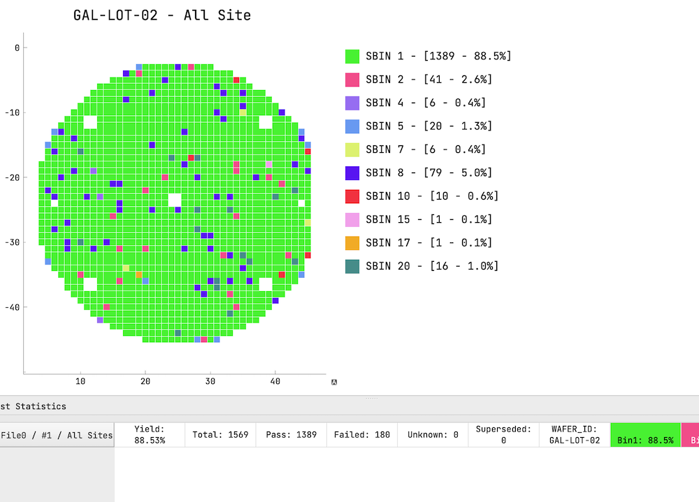
| CP white/dark pixel map | 電性/光學 fail 在 die 與 wafer 上的空間分布 | 只有 bin map 就能分辨是 DTI damage、implant、metal、micro-lens 或測試條件 |
| 可能製程機制 | 可能 inline/形貌訊號 | 還要補的下游證據 |
|---|---|---|
| Etch residue/micromasking | 局部 particle、trench 口異常、cluster/chamber signature | Review SEM/TEM、元素分析、chamber/PM commonality、CP pixel map |
| CD/depth non-uniformity | wafer/reticle 系統性 pattern contrast、專用 target trend | OCD/CD-SEM 模型、cross-section、split 與電性/光學 response |
| Sidewall damage/charge damage | 可能沒有強 optical defect,或只見相關製程 signature | 暗電流/hot pixel、電性、TEM/材料分析;不能靠 KLA optical 單獨宣判 |
| Fill void/seam | 視深度、材料與 mode 而定,可能有微弱 contrast 或完全看不到 | e-beam/cross-section/TEM、同座標 correlation 與 split verification |
同 layer、同 recipe revision、同 scan area/sampling、同 tool/channel,再比較 total;條件不同就先看 density 或重新對齊條件。
total 高但全是已知 nuisance,和 rare killer class 增加是兩件事。Review Count 本身不能代表母體,要看 sampling rule 與 class proportion。
監控間隔決定 at-risk lot 範圍;越疏的 monitor 會讓一次 excursion 需要圈更寬。
做 pre/post map、repeater、tool/chamber/recipe/PM commonality,區分 incoming、process adder 與量測假象。
先圈 last-good/first-bad、在製與已出貨 exposure;定義 hold、加量測、tool stop/chamber hold 與 owner。
先寫清楚要看到哪些 qual/recheck/downstream 結果、多少 wafer/lot、由誰 sign-off 才能解除。
Total candidates、去重後事件、還是 reviewed sample?
有效 scan area、die sampling 與 recipe revision 是否相同?
class mix、map signature、review confidence 怎麼變?
技術主張優先使用 KLA 官方頁、新聞稿、KLA 專利與共同作者論文;專利說明「可採用的方法」,不等於每台量產機、每個 recipe 都啟用全部方法。
查證日期:2026-07-21。產品能力以公開頁可證實內容為界;專利代表可採用的方法,不代表每台量產機/recipe 全部啟用。Fab 內部的機型 option、欄位名稱、scan area、threshold、sampling 與 release spec 仍要回到 data dictionary/SOP。
Load/recipe → align/height → swath/TDI → calibration/registration → reference/fusion → threshold → de-duplicate/cluster → map/KLARF → review;另含工具家族、近年演進、noise、指標與 CIS evidence chain。
你們機型與 option、recipe mode、pixel size/swath、care area、scan area 定義、DDR 欄位、review sampling rule、ADC class tree、baseline/SPC spec。